Sage/DREAM Breast Cancer Challenge Launch

This morning's webinar marked the public launch of the Sage/DREAM Breast Cancer Challenge.  The goal is simple:  given a large data set consisting of clinical covariates, copy number data, expression data, and survival data, can you produce the best predictions of survival time for new patients?  The unstated goal is a little bit more subtle:  so far, there is no compelling evidence that I have seen that microscopic information such as gene expression or copy number data adds anything to predictive power in macroscopic behavior such as the survival time of the patient.  We hope that this competition will encourage people to build better models of disease collaboratively, and produce some of the first evidence that gene expression and copy number data can actually be useful in predicting patient prognosis.  As an example, I will produce an entry that you can feel free to cannibalize, and will write more about it as I evolve it into a better model of disease.  As a Sage employee, I am not eligible to win and so I hope you will modify and adapt this code and produce your own entry, superior to my own!

Before trying my code, you will want to check out the Breast Cancer Competition Getting Started Guide.

From an internal competition we ran that preceded this launch, we learned that the R RandomSurvivalForest package produced the best models of survival given the data, and that in fact the most critical part of the model was actually which data is chosen for inclusion and how it is pre-processed before being handed over to RandomSurvivalForest.

First, I will produce the core of my submission, the model class file.  I will take only the clinical covariates and totally ignore the copy number and expression data, though I will leave a space where they can be included later.  In fact, you will find that this transformation function is the most important part of the entire competition:  victory will hinge not on the best model, but instead on cleaning up the data in the best way possible.

View my Model Class File on github.

Next, I will train and submit the model.  This code is relatively straightforward, but if you are going to modify my model for your own purposes, you will want to make sure that you submit to the public leaderboard instead of the Sage leaderboard!

View my Submission File on github.

As you can see, my Random Survival Forest Clinical-Only model did pretty well!  On the Sage employees leaderboard, model "Sauerwine RSFModel test 3" got a respectable test score of 0.71.  In my next post, we'll see how to improve that further.  At the time of this post, it actually does better than any model on the Sage/DREAM Public Leaderboard, but since you're free to take my model and improve on it, that's not likely to be the case for long!

Good luck, and happy modeling!

Keep it Simple!

I've updated my CV to reflect some success I've had lately in TopCoder Marathon Matches.  I competed in the Harvard Medical School #3 Competition, where I did dismally, and the NASA Tournament Lab "SynchronousControl" Weekend Competition, where I got a 4th place award.

I learned a lot from these contests, so I'll comment a bit on how they went and how I could have improved.

In the HMS #3 Competition, users were asked to examine simulated gene marker time series data to determine which genes were being most strongly selected for and against.  This boiled down to doing a regression on some data points from a Markov chain, and trying to determine what the parameters of the Markov chain were.  In principle, it was actually pretty straightforward.  Simply returning "parameter = (x1-1)/x0" actually did pretty well--better than my solution!  I had tried several different and more advanced regressions, as well as methods to try to account for uncertainty on the data points.  Ultimately, it turns out that all of this complex math did slightly worse than the obvious solution stated above.

The question itself had some problems, in my mind.  First, they assume that the reading at any given time point was correct and free of noise for the purposes of the next iteration of the Markov chain.  Second, the nature of the problem was such that you could not nominate a gene for being both a "most up-regulated" and "most down-regulated" gene.  Sometimes, the noise turned out to be so extreme that my best guess would have been to nominate a gene for both categories!  Finally, the simulated data was modified so that no gene would ever have a reading of zero, which is not realistic given the nature of the experiment.  So, I'm not entirely certain that the researchers who ran the contest are ultimately going to find that the solution is what they actually wanted in the first place.

What I should have done, in retrospect, is the following:  First, I should have immediately dissected and worked backwards from the data simulation program.  The problem description was not exactly representative of the way the data was being simulated, and understanding this earlier certainly would have affected my progress.  Simulating a lot of my own data for my own test harness also would have been instrumental.  Second, I found that very complex methods are actually not all that much better than very simple methods.  I should have taken all of the simple models I tried and compared them in parallel to simulated data and understood the domains in which each model worked the best, then attempted to identify the domain that each data set was in and used the best simple model per task.

So, I say that I did "dismally" because the extremely complex model I settled on was embarrassingly worse than the simplest possible model.

To be fair, the NTL competition that I got a 4th place award in didn't go a lot better.  The problem was to determine what moves to make to help a bunch of robots escape from a maze, under the condition that all of the robots must make the same set of moves!  The principal challenge was that the program to find these moves had to complete in under 2 seconds, which left time for just one A* or BFS in the largest possible map.  I spent way too much time working on a solution that I had to discard because it performed more searches than could be conducted in 2 seconds.

If I had realized this earlier, I would have focused on a heuristic to help robots cooperatively reach their goals instead of focusing on ways to greedily get each robot out individually in the best time.

The algorithm I ultimately used was this:  "Identify the closest robot to any goal.  Perform the minimum number of moves to get that robot out."  This crude method was sufficient to get a 4th place award in my room, $50.  What I would have done if I had to do it again would be this:  "Identify the closest robot to any goal.  Perform the move that minimizes the average distance between all robots and any goal, subject to the constraint that the closest robot must either move closer or stay the same distance away."

The overall lesson was this:  keep it simple.  I often find myself gravitating towards some complex custom algorithm which may either grossly overfit in the case of the HMS competition or may spend way too much processor time grinding away towards a solution when a crude heuristic could have approximated a better solution much more quickly.  When working on these open-ended problems, I need to fight the urge to write a complex algorithm, stay focused on the goal, and home in on the best solution using increasingly better heuristics.

Vacation: Olympic National Rainforest

For her birthday, I flew my friend Lilli over to Seattle to explore the Olympic National Rainforest.  I'd seen pictures of the idyllic mosses and glaciers near the Hoh river, and I must say that it's something you have to see in person.  The forest is incredibly lush and green, but it's often hard to take a good picture because it seems like something is always in the way of your shot, and it was difficult to find wildlife because there were way too many hiding spots.  To make matters worse, I grossly underestimated how cold it got there at night, and overestimated how waterproof my tent would be.  I'll have to try to make the 18 mile hike up to the glacier meadows some other time!  The park as a whole is wonderfully maintained, and the rangers and park staff were pleasant and helpful--just make sure you come prepared for the moisture, cold nights, and permethrin-resistant mosquitoes.

A columbine flower, Aquilegia formosa

Scaphinotus angusticollis looking for a meal on a mossy trunk.

The elk were quite unafraid of people.

The trees frequently had hollow openings under them.  This effect occurs because the only sunlit real estate on the forest floor is where another tree has recently fallen!  This tree began its life growing on the trunk of a fallen predecessor, and now that progenitor has rotted away.  

What Is the Most Dangerous Drug?

The recent Miami cannibal attack brought "bath salts" to the attention of the general public.  Bath salts are not the Epsom salts that sit unused in bathrooms nationwide, but are actually designer drugs that are sold as bath salts in order to circumvent regulation of the component chemical (typically MDPV) and avoid legal responsibility for the results of human consumption.  These designer drugs are frequently legal for possession or consumption since they are not controlled substances, but instead are chemically similar to controlled substances on the theory that similar chemicals should have similar recreational effects.

While reading about these so-called "research chemicals" at Erowid, a project that purports to provide honest information about drug effects and dosage for users and health care providers, I became interested in the stories of user experiences with these poorly-understood substances.  Assessing the similarities and differences between user accounts, it appeared that despite the small sample size there were indeed typical presentations of the effects of each drug.  If the thematic saturation from just a dozen or so accounts were enough to assemble a list of common experiences and side effects, then given the enormous number of user accounts at Erowid can I draw some conclusions about the relative danger of drugs in spite of the obvious self-selection bias?  A few notes before I start:

• I will discard all drugs with fewer than 100 total user accounts from my study.  If you would like to repeat this study from the R code with a different threshold, source is provided.
• The reports at Erowid are self-selected.  For example, you will see in Table 2 that alcohol use is less reported than cocaine.  Obviously, a smaller proportion of alcohol users see fit to report their experiences than cocaine users since most adults drink alcohol.  I cannot account for this self-selection bias, and it certainly taints all of my results.
• Data is collected from all user accounts at Erowid on June 27, 2012.
• I have made the R code for this web scraping experiment available here.  It includes web scraping code, an example of elastic net models in R with the glmnet package, labeled scatterplots, and how to produce normalized word cloud data.
• The dose makes the poison, and I haven't done anything to account for the size of the dose nor the method of drug delivery.  Each case in Erowid should be considered a recreational or abusive dose.  
• I in no way account for "fatally bad experiences" versus just "didn't enjoy it."  You will learn below that the risk for caffeine is quite high because the users take absurdly high amounts of it and are merely uncomfortable during the experience.  There are other drugs where a high dose will do far worse than make you uncomfortable.
• There is no intrinsically safe substance.  None of these results should be construed as an endorsement of any illegal drug use.

First, I used Erowid's search feature to retrieve all user experiences, the drugs that were taken during the session, and the category of report.  I assembled these into large binary matrices, where the category of the report is the response variable and the drugs taken were the features.  I did not discriminate between large and small doses, and only counted whether or not a drug was taken at all during an experience.

Next, I decided to group the response variables a bit more coarsely. In my study, I will refer to number of reports, reward, risk, and addictiveness.

Table 1:  Categories of experiences in my study versus Erowid.

My Study	Erowid Category
Number of Reports	Total number of data points in all categories
Reward	"Glowing Experiences", "Mystical Experiences", "Health Benefits"
Physical Risk	"Health Problems", "Train Wrecks & Trip Disasters", "Addiction & Habituation"
Addictive	"Addiction & Habituation"

Finally, I will build an elastic net model to determine which drugs are most associated with each category.  Because the majority of experience reports at Erowid involve a cocktail of drugs, it is necessary to use a predictive model that will be able to give me some idea as to the risks of individual elements when several are taken together.  In R, the code looks like this:

require(glmnet)
rewardModelGLMNET <- glmnet(featureTable, rewardTable, family="binomial")

This is all that is required to extract coefficients for each of reward, risk and addictiveness.  I present the coefficients in a model using all of the drugs with at least 100 experiences in Table 2.

Table 2:  Reward, Risk, Addictiveness and number of reports of drugs from Erowid.  Unitless model coefficients are given, which gauge the relative reward, risk or addictive nature compared to other drugs on the list.  Note the obvious self-selection bias visible in the list of reported drugs, where cocaine and opiates are ranked more highly than the relatively ubiquitous alcohol. 

Most Rewarding DMT 0.94 Ayahuasca 0.89 Cacti 0.83 2C-I 0.79 Mushrooms 0.76 Pharms - Paroxetine 0.72 MDMA 0.72 Nitrous Oxide 0.62 5-MeO-DMT 0.52 Morning Glory 0.48 Methylone 0.45 H.B. Woodrose 0.43 DPT 0.4 Hydrocodone 0.39 AMT 0.36 LSD 0.32 Salvia divinorum 0.29 Mimosa spp. 0.28 Kava 0.27 Kratom 0.26 2C-E 0.25 2C-T-2 0.23 Harmala Alkaloids 0.22 Melatonin 0.22 Ketamine 0.21 2C-B 0.16 Opioids 0.13 Pharms - Buprenorphine 0.12 Cannabis 0.11 Pharms - Venlafaxine 0.08 Modafinil 0 Pharms - Alprazolam -0.02 Pharms - Tramadol -0.02 2C-T-7 -0.05 Heroin -0.05 Anadenanthera spp. -0.07 Pharmaceuticals -0.07 5-MeO-DiPT -0.12 Pharms - Clonazepam -0.12 Amphetamines -0.12 Tobacco -0.13 Pharms - Oxycodone -0.24 Opiates -0.27 Amanitas -0.31 Alcohol -0.33 Benzodiazepines -0.33 Syrian Rue -0.34 Pharms - Methylphenidate -0.41 Codeine -0.42 Cannabinoid Receptor Agonists -0.43 Methamphetamine -0.51 Pharms - Bupropion -0.54 Absinthe -0.57 GHB -0.6 DXM -0.6 Spice and Synthetic Cannabinoids -0.78 Nutmeg -0.82 Pharms - Zolpidem -0.82 Cocaine -0.84 Datura -0.95 Caffeine (extreme dose) -0.98 5-MeO-AMT -1 Inhalants -1.1 Piperazines -1.1 SSRIs -1.12 Diphenhydramine -2.01 Dimenhydrinate -2.44 Least Rewarding

Most Risky GHB 1.62 Methamphetamine 1.51 Heroin 1.35 Cocaine 1.16 Pharms - Venlafaxine 1.15 Inhalants 1.09 Opioids 0.93 Tobacco 0.91 Caffeine (extreme dose) 0.9 Syrian Rue 0.85 Pharms - Buprenorphine 0.82 Amphetamines 0.76 Pharms - Tramadol 0.73 Pharms - Paroxetine 0.69 Pharmaceuticals 0.68 DXM 0.64 Alcohol 0.48 Datura 0.47 Pharms - Zolpidem 0.45 Dimenhydrinate 0.42 Pharms - Methylphenidate 0.4 Diphenhydramine 0.38 5-MeO-AMT 0.32 Benzodiazepines 0.25 Nitrous Oxide 0.2 Opiates 0.19 AMT 0.18 MDMA 0.16 Pharms - Bupropion 0.13 SSRIs 0.1 2C-T-7 0.05 Piperazines 0.02 Kratom -0.01 Modafinil -0.08 Pharms - Oxycodone -0.11 Pharms - Alprazolam -0.15 Spice and Synthetic Cannabinoids -0.16 Cannabis -0.19 Cannabinoid Receptor Agonists -0.2 Ketamine -0.22 LSD -0.29 Codeine -0.3 Morning Glory -0.32 Amanitas -0.39 Pharms - Clonazepam -0.39 5-MeO-DMT -0.42 Nutmeg -0.5 Hydrocodone -0.5 DPT -0.53 5-MeO-DiPT -0.63 H.B. Woodrose -0.65 2C-T-2 -0.7 Harmala Alkaloids -0.73 Melatonin -0.76 2C-E -0.78 Methylone -0.83 2C-B -0.85 Kava -0.92 Ayahuasca -0.93 2C-I -0.94 Mushrooms -1.02 Mimosa spp. -1.09 Anadenanthera spp. -1.27 Absinthe -1.31 DMT -2.14 Cacti -2.17 Salvia divinorum -2.19 Least Risky

Most Addictive Methamphetamine 2.21 Cocaine 2.05 Opioids 1.53 Pharms - Buprenorphine 1.46 Heroin 1.43 Pharms - Venlafaxine 1.38 Amphetamines 1.33 Tobacco 1.31 Pharms - Paroxetine 1.26 Pharms - Tramadol 1.2 GHB 1.08 Pharms - Methylphenidate 0.93 Opiates 0.67 Benzodiazepines 0.67 Kratom 0.65 Pharms - Clonazepam 0.65 Inhalants 0.55 Caffeine (extreme dose) 0.52 Nitrous Oxide 0.39 Pharms - Alprazolam 0.3 Modafinil 0.07 DXM 0.03 Pharms - Zolpidem -0.03 Ketamine -0.08 Pharms - Bupropion -0.1 Alcohol -0.15 Pharms - Oxycodone -0.16 MDMA -0.16 Dimenhydrinate -0.22 Diphenhydramine -0.26 Cannabinoid Receptor Agonists -0.3 Pharmaceuticals -0.31 Codeine -0.45 Harmala Alkaloids -0.51 Methylone -0.52 Cannabis -0.67 Melatonin -0.81 Absinthe -0.83 Hydrocodone -0.83 5-MeO-AMT -0.88 SSRIs -1.04 2C-T-2 -1.23 Piperazines -1.24 Spice and Synthetic Cannabinoids -1.28 5-MeO-DMT -1.54 Kava -1.64 AMT -1.7 2C-E -1.83 Datura -1.85 LSD -1.88 2C-T-7 -2.16 5-MeO-DiPT -2.31 DPT -2.32 Mushrooms -2.86 Mimosa spp. -3.35 Syrian Rue -3.81 Salvia divinorum -3.87 Ayahuasca -4.88 Anadenanthera spp. -5.03 Amanitas -5.38 Cacti -5.43 DMT -5.49 H.B. Woodrose -5.6 Nutmeg -5.7 2C-B -5.7 Morning Glory -5.82 2C-I -5.96 Least Addictive

Most Reported Experiences Mushrooms 1839 Cannabis 1637 Salvia divinorum 1577 MDMA 1354 LSD 1232 DXM 730 Opiates 589 Pharmaceuticals 582 Opioids 544 Cocaine 529 Alcohol 491 Morning Glory 463 2C-I 458 Amphetamines 425 Harmala Alkaloids 414 Methamphetamine 353 5-MeO-DiPT 318 DMT 315 Ketamine 314 5-MeO-DMT 310 SSRIs 305 H.B. Woodrose 304 Syrian Rue 301 2C-E 292 Datura 291 Nutmeg 289 AMT 274 Nitrous Oxide 258 Cacti 256 Diphenhydramine 248 Benzodiazepines 236 2C-T-7 235 Pharms - Tramadol 232 2C-B 229 Caffeine (extreme dose) 213 Kratom 209 Dimenhydrinate 207 Pharms - Oxycodone 205 Amanitas 194 Hydrocodone 194 Heroin 191 DPT 185 Inhalants 185 Ayahuasca 179 GHB 172 Kava 172 Pharms - Zolpidem 165 2C-T-2 164 Codeine 161 Pharms - Alprazolam 150 5-MeO-AMT 138 Pharms - Methylphenidate 138 Mimosa spp. 136 Tobacco 132 Pharms - Bupropion 128 Pharms - Paroxetine 124 Pharms - Venlafaxine 124 Modafinil 111 Methylone 109 Absinthe 108 Anadenanthera spp. 107 Melatonin 105 Spice and Synthetic Cannabinoids 104 Pharms - Buprenorphine 101 Piperazines 98 Pharms - Clonazepam 96 Cannabinoid Receptor Agonists 90 Least Reported Experiences

Table 2 gives lists of the most rewarding, risky, addictive and most reported common drugs on Erowid.  I found it interesting that the most rewarding and least addictive drugs tended to be hallucinogens and entheogens, and that the most stereotypically abused drugs (cocaine, heroin, methamphetamine) had higher risk and addiction coefficients but generally lower rates of rewarding experiences. This trend makes me think of the Rat Park Experiment where it was shown that rats that lived happy lives did not become addicts despite easy availability of drugs in their environment.  This supports the idea that methamphetamine, cocaine, and heroin may indeed be more of an avenue of escape than a positive experience in their own right.  The bath salts which I wondered about from the cannibal attack in the news typically contain MDPV, a substance which did not have enough documented experiences on Erowid to pass my criterion for inclusion of having more than 100 user reviews.  

Figure 1:  Risk versus Reward in common drugs on Erowid as calculated by an elastic net model.  Please note that this plot is greatly affected by self-selection bias.  For example, normal users of caffeine think nothing of it, but do not report their experiences.   

Most remarkably, Figure 1 shows that the risk-to-reward ratio of hallucinogens and entheogens tended to be in the "more rewarding, less risky" category, and drugs categorized as research chemicals tended to offer a better reward-to-risk ratio than alcohol, tobacco, cocaine or heroin.

Overall, I was a bit disappointed with the results of this study.  Not shown are numerous plots and statistics that I thought would be enlightening, but in the end were worthless due to the corruption of the self-selection bias.  For example, I was sure there would be a correlation between number of reports and reward coefficient, but in fact I could find nothing significant.  It's possible that availability is a bigger factor in selecting a drug than reward, or that users of some drugs are simply more inclined to share their story.  In order to get better data on the effects of illegal drugs, it would require a survey designed to avoid self-selection bias.

In conclusion,

• This study was enormously biased.  The popularity section of Table 2 shows a colossal self-selection bias because cocaine is reported far more than alcohol.  I did not account for dose nor for the type of risk, which is obvious because high doses of caffeine were more associated with risk than alcohol.
• There was not enough data at Erowid to satisfactorily assess the outcomes associated with MDPV, a principal component of many "bath salts".  The R code for this study is provided in case you would like to check for yourself with another threshold.
• The user experiences at Erowid indicate that that the most rewarding and least risky drugs tend to be hallucinogens and entheogens.  
• The user experiences at Erowid indicate that the most dangerous drug is GHB, followed by Methamphetamine, Heroin and Cocaine.
• I do not partake in, endorse or recommend the use of any illegal substance.  There is no intrinsically safe substance.      

As a bonus, I added some code to the R script to produce word cloud data for use with programs such as the freeware program Wordaizer.  To produce these word clouds, I first counted all of the words in a random sample of Erowid experiences, then counted the words in the experiences of just the drug of interest.  By dividing the frequency of each word in the drug-specific set by the frequency of each word in the control sample, I was able to get an idea of which keywords were truly more common and unique to each drug as opposed to Erowid experiences in general.  I then used Wordaizer under Wine in order to produce these attractive word clouds.  The code I used to produce these is freely available.

Ayahuasca	Caffeine	Cannabis
GHB	Inhalants	LSD
Cocaine	Heroin	Meth

Figure 2:  Word clouds produced using Wordaizer with Erowid experiences for a selection of drugs, normalized and prepared with R code available above.

Thanks to Simiao for proofreading and advice regarding the design of this study.  

Are Campaign Slogans Getting Shorter?

In 2008, Americans elected a president whose slogan was the shortest ever, both in terms of syllables and length:  "Hope."  I wonder:  have US presidential campaign slogans gotten shorter?  Perhaps a low level of public interest in American politics and decreasing attention spans together have led to the public favoring the candidate with the shortest slogan.

In US history class I learned about the revolutionary "I Like Ike" campaign ad.  Television was a relatively new medium in the 1950s and was just beginning to see widespread adoption, and the commercial featured a catchy tune that stuck in your head, a short slogan, and visuals that subtly reminded you of Eisenhower's credentials.  Maybe each advance in media has further decreased Americans' attention span, and as such slogans have kept getting shorter each year until we hit the information limit of one syllable and four letters in 2008.  To address my question, I pulled a list of 200 US presidential campaign slogans from tagline guru, removed all of the "anti-" slogans, and then for each remaining entry marked whether or not that campaign was successful and how many syllables were in the slogan.  If slogans have indeed gotten shorter, then I should see a negative trend in their length over time.

Figure 1:  Syllable (left) and Character (right) length of US presidential campaign slogans.  Winning campaign slogans are in green, losing in red.  If multiple slogans were used by the same candidate in the same campaign, then all are included.  

Figure 1 shows scatter-plots of syllable and character length of US presidential campaign slogans versus year.  I have not included trend lines, because the scatter is obviously so great that the result wouldn't be particularly meaningful.  The length of successful or unsuccessful presidential campaign slogans does not appear to have changed much across the last two centuries of US history.

Figure 2:  Histograms of  syllable (left) and character (right) length of US presidential campaign slogans.  Green represents winning slogans, red represents losing slogans.

In figure 2, I have produced a chart of the relative frequency of each slogan length hoping to find some evidence that Americans have historically had some preference of shorter versus longer slogans.  In fact, a t-test indicates that the average winning slogan has on average 7.35 syllables and the losing slogans have on average 6.51 syllables, with p=0.05 (this means that the probability that the means of these distributions are actually the same, and this result occurred from random chance alone, is 0.05, or 1 in 20).  On the other hand, the average winning slogan has 25.7 characters and the average losing slogan has 23.6 characters, with p=0.15.  The large p-values and the similar means indicate that there is probably no preference between longer and shorter slogans.  If there is a preference, however, it is in favor of longer slogans!

So, US presidential campaign slogans have on average remained the same length throughout American history, and there is weak evidence (p=0.05) that Americans prefer syllabically longer campaign slogans to shorter ones.

The Cob-Web

While doing some web scraping for another project, I collected some ancillary data that I think you'll find interesting.  I wrote a program to  collect a comprehensive list of .com top level domains, and I wondered:  how many .com domains are there?  How long is the average domain?  The longest?  Roughly what proportion of them are parked, typical websites, or pornography?

The answer, I thought, was actually pretty sad.  The web that I had been led to believe was predominantly pornography and parking was actually mostly abandoned.  In my simple random sample, there were more parked domains than all other non-404 websites combined.  I'll get to that in a bit.  Please note that this study only concerns .com domains, not .net, .org, .gov, .edu, or anything else.


Let's start by taking a look at the distribution of domain name lengths.  Since my data file included the ".com" part, but not the "http://" part, I could parse out the domain name proper with a simple one-liner in bash:

awk '{print length($1)-4}' domainList | sort -n | uniq -c | awk '{print $2, $1}'

Figure 1:  Two views of the number of registered .com domains versus the length of the domain name.  Note the logarithmic scale on the left.  

Remarkably, there were only three registered one-letter domain names:  q.com, x.com and z.com (these must be grandfathered in), and z.com returned a 404 error.  There were available and unregistered 2-letter domain names, and there were at least a million domains having each length from 5-21.  The most common domain name length was 11, and there were 547 .com domains with the maximum length of 63 characters.  I counted 54,816,663 registered dot-com domains total on April 30, 2012.

Now I wanted to get a handle on what the landscape of the web looked like.  I used another simple one-liner to generate a list of 100 randomly selected domains from my collection:

awk '{print rand(), $1}' domainList | sort -n -k 1 | head -n 100 | awk '{print $2}'

I acted as my own Mechanical Turk, classifying each of the 100 domains in my simple random sample as either 404, parked, XXX, website placeholder, or website.  Website placeholders were purchased, but never developed and displayed a message from the registrar.  A 95% confidence interval is given for each type.

Type of .com	Proportion (95% CI)
404	48 ± 9.8%
Parked	28 ± 8.8%
'Normal' Website	19 ± 7.7%
Placeholder	4 ± 3.8%
'XXX' Website	1 ± 1.9%

Table 1:  Types of website, and proportion in my n=100 random sample.

Table 1 gives a surprising view of our web:  about half of it returns a 404 error.  About a quarter of it is parked by people seeking to make an easy buck by re-selling the domain.  About a fifth is what we would consider a website, and the remainder is either a placeholder where someone will ostensibly develop a new website or pornography, which is actually apparently quite rare compared to typical personal or corporate web pages.

Though the error bars are quite large (admittedly, I tired of being a Mechanical Turk), this exercise challenged my stereotype of the web.  This shows that there is a huge amount of turnover where domains are relinquished and picked up, mostly by domain parking speculators but also by legitimate people and businesses.    It also raises another concern:  if a website can be considered part of the culture of the information age, what is happening to the enormous amount of information and data that is being turned over?  The internet archive has put forth a valiant effort, but nonetheless websites disappear like the great cities of the past, except without any ruins that future historians could ever hope to dig up and analyze.

It may prove that the information age has a very short memory!

How Fast is My Internet Connection, Actually?

A series of tubes.

When diagnosing the speed of my internet connection, I'd been using online speed tests such as speedtest.net to determine what sort of bandwidth I was getting.  I lamented, however, that these were single data points and as such were not sufficient to say one way or the other whether or not my ISP was actually network-neutral or whether I was getting this speed at all times.  Further, since cable internet is a shared line, I'd like to know what the fluctuation in bandwidth over a day looks like.

I found the open-source suite NeuBot, which uses a distributed network of speed test servers as well as BitTorrent peers to periodically test my connection speed and determine what my bandwidth is over time, which is certainly a much better measure than the single data points offered by most simple online bandwidth tests.

First, some details about my setup:

• I have the Comcast/Xfinity Blast plan, which offers 20Mbps down and 4Mbps up, and actually a bit faster considering the "PowerBoost" feature which provides 20% more speed for the first 20MB of a file down, and 10MB up.
• I am using an Arris TouchStone WBM760A and a Linksys WRT54GL router.
• When testing the wireless connection, I put my desktop wireless antenna next to the router.
• I did not in any way control for what else I may have been doing on the network at the time.

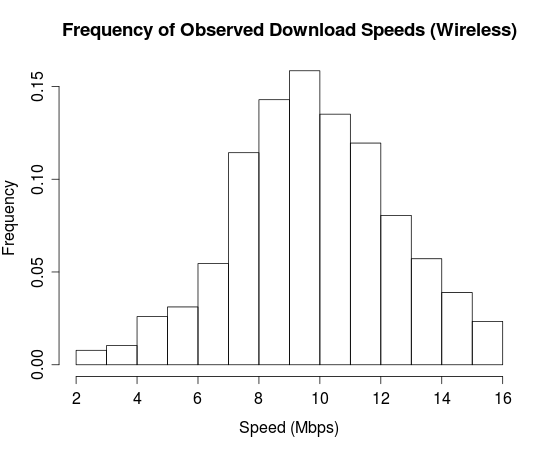
Since my router claims to support speeds up to 54Mbps, let me now compare my connection speeds while on wireless to those on the wired connection.  I copy and pasted the data out of Neubot, and ran the following lines of R:

data <- read.table("~/Desktop/speedtest-wired.dat")

hist(data[,10], freq=FALSE, main="Frequency of Observed Download Speeds (Wired)", xlab="Speed (Mbps)", ylab = "Frequency")
hist(data[,12], freq=FALSE, main="Frequency of Observed Upload Speeds (Wired)", xlab="Speed (Mbps)", ylab = "Frequency")

Figure 1:  Upload and Download speeds on Wired and Wireless connection with the Linksys WRT54GL.

Intriguingly, my "54 Mbps" Linksys router is not able to provide nearly the promised download speed on the wireless.  On wireless, it provided an average of 9Mbps down and reasonable performance up, whereas on the wired connection my connection speeds were just as promised down, and perhaps a bit slow at about 3.5 Mbps up.  Since the download speeds on the wireless look Gaussian, I am led to believe that this is due to interference from local sources such as other wireless networks.

Now let's see if I can detect throttling of BitTorrent.  Neubot tests both BitTorrent as well as a conventional speed test, and so if the connection is net-neutral, I expect to see very similar speeds both down and up.

Figure 2:  Upload and Download speeds for normal speed tests versus BitTorrent upload and download speeds.  

While the upload and download speeds for BitTorrent appeared quite a bit more noisy than those for the normal speed test, the results are quite similar with the most noticeable difference being the long tail of slower upload speeds for BitTorrent.  It would require data from considerably more computers to make a case for this being throttling of BitTorrent connections, and so I have contributed my data to the collection being amassed by the NeuBot project.  

Now let's look at how my connection speed varies throughout the day.  Since cable internet connections are on a shared line, I should see my connection speed reduced during peak times of use.  I used the following R to generate these plots:

require(gplots)
require(foreach)

errbars <- function(x, y) {
  mygroups <- unique(x)

  groups <- foreach(i = 1:length(mygroups)) %do% {return(y[x==x[i]])}
  
  yavg <- unlist(lapply(groups, mean))
  ystdv <- unlist(lapply(groups, sd))

  return(list(x=mygroups, lo=yavg-ystdv, yavg=yavg, hi=yavg+ystdv))
}

bars <- errbars(as.numeric(regmatches(as.character(data[,2]), regexpr("[[:digit:]]+", as.character(data[,2])))), data[,10])
plotCI(bars$x, bars$yavg, ui=bars$hi, li=bars$lo, xlab="Hour of Day", ylab="Observed Download Speed (Mbps)")


Figure 3:  Variation in wired connection speeds throughout the day.  Error bars are one standard deviation. 

Connection speeds appeared to be remarkably stable throughout the day, and clearly more data would be necessary in order to see any significant difference between the speeds at various times.  This data was collected over two weeks, and there were about 20 data points per hour.  Suffice it to say that if there is variation in my connection speed throughout the day, it is not very large, no more than 2Mbps down and perhaps 250Kbps up.

This exercise tested my internet connection speed systematically, and I found nothing lacking in Comcast/Xfinity's service.  In particular, I learned the following about my connection:

• Despite the label saying that my Linksys WRT54GL router supports 54Mbps connection speeds, it is unable to deliver even 20Mbps over wireless.  The Gaussian connection speed profile in figure 1 leads me to believe that there is some interference confusing it.  
• The median connection speeds for the normal speed test and BitTorrent test are both nearly the same as my advertised connection speed, indicating that Comcast/Xfinity is not throttling BitTorrent in any noticeable fashion.
• My internet connection speed did not change significantly throughout the day, which is surprising given that I am on a line shared with everyone in my building and perhaps some neighboring buildings.  Perhaps this accusation which is leveled at cable internet providers by fiber and DSL providers is unfair.

I encourage you to install NeuBot yourself and put your own ISP to the test!

Thanks to L D Christoph for allowing me to use her connection as a control group.